Exercise potential energy statically indeterminate structure

Exercise potential energy statically indeterminate structure#

Find the displacement in C using potential energy and compare it to the result from solving the differential equation.

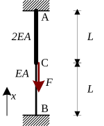
../_images/structure7.svg — Fig. 1 Structure#

Solve using potential energy#

Let’s start by defining the trial function. Let’s assume a parabolic displacement field with the shape \(u\left(x\right) = a + b x + c x^2\).

Exercise (Boundary conditions kinematical admissible trial function)

The displacement field must be kinematically admissible. Which boundary conditions must be enforced for that?

Solution to Exercise (Boundary conditions kinematical admissible trial function)

\(u\left(0\right) = 0\)
\(u\left(2L\right) = 0\)

Exercise (Kinematical admissibility trial function)

Now, let’s use SymPy to rewrite the trial function so that it is kinematically admissible.

import sympy as sym
a, b, c, x, L, EA, F = sym.symbols('a, b, c, x, L, EA, F')

u_trial_general = a + b * x + c * x **2

eq1 = sym.Eq(u_trial_general.subs(x, #value to substitute for x), #right hand side of equation)
eq2 = #...
sol = sym.solve((eq1,eq2),(a,b))
display(sol)
u_trial = u_trial_general.subs(sol)
display(u_trial)

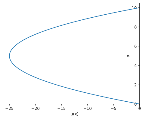
Let’s check your solution graphically for a value of \(1\) for \(c\) and \(5\) for \(L\):

import matplotlib.pyplot as plt
import numpy as np
%config InlineBackend.figure_formats = ['svg']

%matplotlib inline
u_trial_func = sym.lambdify(x, u_trial.subs(sol).subs(c,1).subs(L,5))
x_plot = np.linspace(0, 10,100)
fig, ax = plt.subplots()
ax.plot(u_trial_func(x_plot),x_plot)
ax.spines['right'].set_color('none')
ax.spines['top'].set_color('none')
ax.spines['bottom'].set_position('zero')
ax.spines['left'].set_position('zero')
ax.set_xlabel('u(x)')
ax.set_ylabel('x')
fig.patch.set_alpha(0.0)
ax.patch.set_alpha(0.0)

Solution to Exercise (Kinematical admissibility trial function)

The answer should be \(-2 \ L \ c \ x + c \ x^2\) and the graph should match your boundary conditions of exercise on boundary conditions kinematical admissible trial function

import sympy as sym
a, b, c, x, L, EA, F = sym.symbols('a, b, c, x, L, EA, F')

u_trial_general = a+b*x+c*x**2

eq1 = sym.Eq(u_trial_general.subs(x,0), 0)
eq2 = sym.Eq(u_trial_general.subs(x,2*L), 0)
sol = sym.solve((eq1,eq2),(a,b))
display(sol)
u_trial = u_trial_general.subs(sol)
display(u_trial)

{a: 0, b: -2*L*c}

\[\displaystyle - 2 L c x + c x^{2}\]

import matplotlib.pyplot as plt
import numpy as np
%config InlineBackend.figure_formats = ['svg']

%matplotlib inline
u_trial_func = sym.lambdify(x, u_trial.subs(sol).subs(c,1).subs(L,5))
x_plot = np.linspace(0, 10,100)
fig, ax = plt.subplots()
ax.plot(u_trial_func(x_plot),x_plot)
ax.spines['right'].set_color('none')
ax.spines['top'].set_color('none')
ax.spines['bottom'].set_position('zero')
ax.spines['left'].set_position('zero')
ax.set_xlabel('u(x)')
ax.set_ylabel('x')
fig.patch.set_alpha(0.0)
ax.patch.set_alpha(0.0)

../_images/5ff463e885feb1e2e59c176ded0e3afe4c0b0ba61aff13d9b93f6483b54690cb.svg

Exercise (epsilon)

For the strain energy we needed the strain distribution instead of the displacement. The strain is the derivative of the displacement, which can be found with SymPy:

For this exercise you just have to run the cell below.

epsilon_trial = sym.diff(u_trial,x)
display(epsilon_trial)

Solution to Exercise (epsilon)

You should have found: \(\epsilon \left(x\right) = -2 \ L \ c + 2 \ c \ x \)

epsilon_trial = sym.diff(u_trial,x)
display(epsilon_trial)

\[\displaystyle - 2 L c + 2 c x\]

Exercise (strain energy)

Now let’s evaluate the strain energy:

E_v_trial = sym.integrate(#term to integrate,(x,#integrate from, #integrate to)) + ...
display(E_v_trial)

Solution to Exercise (strain energy)

The answer should be \(2 \ EA \ L^3 c^2\)

E_v_trial = sym.integrate(EA*epsilon_trial**2/2,(x,0,L))+sym.integrate(EA*2*epsilon_trial**2/2,(x,L,2*L))
display(E_v_trial)

\[\displaystyle 2 EA L^{3} c^{2}\]

Exercise (Work by force)

What’s the work done by the force \(F\)?

Solution to Exercise (Work by force)

\[- F \cdot u(L)\]

Exercise (Potential energy)

Find the relation for the potential energy.

V = #expression for V
display(V)

Solution to Exercise (Potential energy)

The answer should be \(2 EA \ L^3 c^2 - F\ L^2 c\)

V = E_v_trial - ( -F * u_trial.subs(x,L))
display(V)

\[\displaystyle 2 EA L^{3} c^{2} - F L^{2} c\]

Exercise (Stationary strain energy)

Now, let’s impose the stationary condition for the strain energy in an equation which we can use to solve for the unknown \(c\).

eq3 = sym.Eq(#left hand side of equation, #right hand side of equation)
display(eq3)
c_sol = sym.solve(eq3,c)[0]
display(c_sol)
u_trial_sol = u_trial.subs(c,c_sol)
display(u_trial_sol)

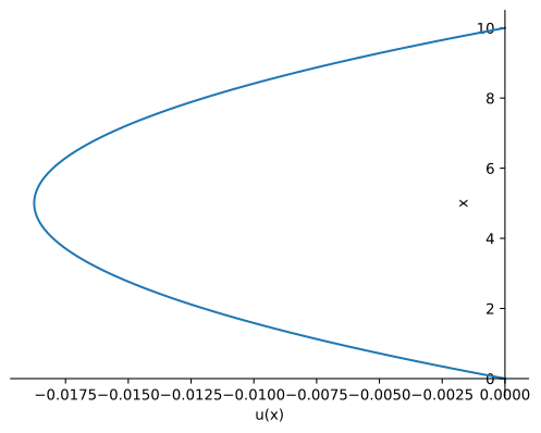
Let’s check your solution graphically for a value of \(5\) m for \(L\), \(2000\) kN for \(EA\) and \(30\) kN for \(F\):

%matplotlib inline
L_test = 5
EA_test = 2000
F_test = 30
u_trial_func = sym.lambdify(x, u_trial_sol.subs(L,L_test).subs(EA,EA_test).subs(F,F_test))
x_plot = np.linspace(0, L_test*2,100)
fig, ax = plt.subplots()
ax.plot(u_trial_func(x_plot),x_plot)
ax.spines['right'].set_color('none')
ax.spines['top'].set_color('none')
ax.spines['bottom'].set_position('zero')
ax.spines['left'].set_position('zero')
ax.set_xlabel('u(x)')
ax.set_ylabel('x')
fig.patch.set_alpha(0.0)
ax.patch.set_alpha(0.0)

Solution to Exercise (Stationary strain energy)

The answer should be \(-\cfrac{F \ x}{2 \ EA} + \cfrac{ F \ x^2}{4 \ EA \ L}\)

eq3 = sym.Eq(V.diff(c),0)
display(eq3)
c_sol = sym.solve(eq3,c)[0]
display(c_sol)
u_trial_sol = u_trial.subs(c,c_sol)
display(u_trial_sol)

\[\displaystyle 4 EA L^{3} c - F L^{2} = 0\]

\[\displaystyle \frac{F}{4 EA L}\]

\[\displaystyle - \frac{F x}{2 EA} + \frac{F x^{2}}{4 EA L}\]

%matplotlib inline
L_test = 5
EA_test = 2000
F_test = 30
u_trial_func = sym.lambdify(x, u_trial_sol.subs(L,L_test).subs(EA,EA_test).subs(F,F_test))
x_plot = np.linspace(0, L_test*2,100)
fig, ax = plt.subplots()
ax.plot(u_trial_func(x_plot),x_plot)
ax.spines['right'].set_color('none')
ax.spines['top'].set_color('none')
ax.spines['bottom'].set_position('zero')
ax.spines['left'].set_position('zero')
ax.set_xlabel('u(x)')
ax.set_ylabel('x')
fig.patch.set_alpha(0.0)
ax.patch.set_alpha(0.0)

../_images/4f684a67006c4ea2fdc3441a2b3b8981e994760f6c7b915346d8dea2a795b91c.svg

Exercise (Normal force)

What is the normal force distribution?

epsilon = #...

N_trial_sol_AC = #
N_trial_sol_BC = #

display(N_trial_sol_AC.simplify())
display(N_trial_sol_BC.simplify())

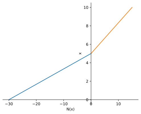
Let’s check your solution graphically for a value of \(5\) m for \(L\), \(2000\) kN for \(EA\) and \(30\) kN for \(F\):

%matplotlib inline
L_test = 5
EA_test = 2000
F_test = 30
fig, ax = plt.subplots()

N_trial_func_AC = sym.lambdify(x, N_trial_sol_AC.subs(sol).subs(L,L_test).subs(EA,EA_test).subs(F,F_test))
N_trial_func_BC = sym.lambdify(x, N_trial_sol_BC.subs(sol).subs(L,L_test).subs(EA,EA_test).subs(F,F_test))
x_plot_AC = np.linspace(0, L_test,2)
x_plot_BC = np.linspace(L_test, L_test*2,2)
ax.plot(N_trial_func_AC(x_plot_AC),x_plot_AC)
ax.plot(N_trial_func_BC(x_plot_BC),x_plot_BC)
ax.spines['right'].set_color('none')
ax.spines['top'].set_color('none')
ax.spines['bottom'].set_position('zero')
ax.spines['left'].set_position('zero')
ax.set_xlabel('N(x)')
ax.set_ylabel('x')
fig.patch.set_alpha(0.0)
ax.patch.set_alpha(0.0)

Solution to Exercise (Normal force)

You should have found:

\(N_{\text{AC,trial}}\left(x\right) = \cfrac{F \ \left(-L + x\right)}{L}\)
\(N_{\text{BC,trial}}\left(x\right) = \cfrac{F \ \left(-L + x\right)}{2 \ L}\)

epsilon = sym.diff(u_trial_sol,x)

N_trial_sol_AC = 2 * EA * epsilon
N_trial_sol_BC = EA * epsilon

display(N_trial_sol_AC.simplify())
display(N_trial_sol_BC.simplify())

\[\displaystyle \frac{F \left(- L + x\right)}{L}\]

\[\displaystyle \frac{F \left(- L + x\right)}{2 L}\]

%matplotlib inline
L_test = 5
EA_test = 2000
F_test = 30
fig, ax = plt.subplots()

N_trial_func_AC = sym.lambdify(x, N_trial_sol_AC.subs(sol).subs(L,L_test).subs(EA,EA_test).subs(F,F_test))
N_trial_func_BC = sym.lambdify(x, N_trial_sol_BC.subs(sol).subs(L,L_test).subs(EA,EA_test).subs(F,F_test))
x_plot_AC = np.linspace(0, L_test,2)
x_plot_BC = np.linspace(L_test, L_test*2,2)
ax.plot(N_trial_func_AC(x_plot_AC),x_plot_AC)
ax.plot(N_trial_func_BC(x_plot_BC),x_plot_BC)
ax.spines['right'].set_color('none')
ax.spines['top'].set_color('none')
ax.spines['bottom'].set_position('zero')
ax.spines['left'].set_position('zero')
ax.set_xlabel('N(x)')
ax.set_ylabel('x')
fig.patch.set_alpha(0.0)
ax.patch.set_alpha(0.0)

../_images/783b96345285484915dd8acbecd9c2f08bf157d391c02b4c9ff30cd42d5ff417.svg

Solve with differential equation#

Now, let’s solve the same structure using the differential equation.

Exercise (Generalised relations)

Given a load \(q=0\), integrate twice to find the normal force, strain and displacement relations with integration constants:

C_1, C_2, C_3, C_4 = sym.symbols('C_1, C_2, C_3, C_4')

q_AC = 0
q_BC = 0

N_AC = C_1 + sym.integrate(#..., x)
N_BC = C_3 + #...

display(N_AC)
display(N_BC)

epsilon_AC = #...
epsilon_BC = #...

display(epsilon_AC)
display(epsilon_BC)

u_AC = C_2 + #...
u_BC = C_3 + #...

display(u_AC)
display(u_BC)

Solution to Exercise (Generalised relations)

You should have found:

\(N_{\text{AC}} = C_1\)
\(N_{\text{BC}} = C_3\)
\(\epsilon_{\text{AC}} = \cfrac{C_1}{2 \ EA}\)
\(\epsilon_{\text{BC}} = \cfrac{C_3}{EA}\)
\(u_{\text{AC}} = \cfrac{C_1}{2 \ EA} x + C_2\)
\(u_{\text{BC}} = \cfrac{C_3}{EA} x + C_4\)

C_1, C_2, C_3, C_4 = sym.symbols('C_1, C_2, C_3, C_4')

q_AC = 0
q_BC = 0

N_AC = C_1 + sym.integrate(q_AC, x)
N_BC = C_3 + sym.integrate(q_BC, x)

display(N_AC)
display(N_BC)

epsilon_AC = N_AC / EA / 2
epsilon_BC = N_BC / EA

display(epsilon_AC)
display(epsilon_BC)

u_AC = C_2 + sym.integrate(epsilon_AC, x)
u_BC = C_4 + sym.integrate(epsilon_BC, x)

display(u_AC)
display(u_BC)

\[\displaystyle C_{1}\]

\[\displaystyle C_{3}\]

\[\displaystyle \frac{C_{1}}{2 EA}\]

\[\displaystyle \frac{C_{3}}{EA}\]

\[\displaystyle \frac{C_{1} x}{2 EA} + C_{2}\]

\[\displaystyle \frac{C_{3} x}{EA} + C_{4}\]

Exercise (Boundary conditions)

What are the boundary conditions?

Solution to Exercise (Boundary conditions)

\(u_\text{AC} \left(0\right)=0\)
\(u_\text{AC} \left(L\right)=u_\text{BC} \left(L\right)\)
\(u_\text{BC} \left(2 \ L \right) = 0\)
\(N_\text{AC} \left(L\right) + F = N_\text{BC} \left( L\right)\)

Exercise (Solve boundary conditions)

Now, let’s use SymPy to solve for the boundary conditions using sym.solve similarly as you did in the exercise for the kinematical admissibility trial function and find the solution for \(u_\text{AC}\), \(u_\text{BC}, \)N_\text{AC}\( and \)N_\text{BC}

eq4 = #...
#...

C_sol = sym.solve((eq4,#...),[#])
display(sol)

u_AC_sol = u_AC.subs(C_sol)
u_BC_sol = u_BC.subs(C_sol)
display(u_AC_sol)
display(u_BC_sol)
N_AC_sol = #
N_BC_sol = #
display(N_AC_sol)
display(N_BC_sol)

Let’s check your solution graphically for a value of \(5\) m for \(L\), \(2000\) kN for \(EA\) and \(30\) kN for \(F\):

%matplotlib inline
u_AC_func = sym.lambdify(x, u_AC_sol.subs(sol).subs(L,L_test).subs(EA,EA_test).subs(F,F_test))
u_BC_func = sym.lambdify(x, u_BC_sol.subs(sol).subs(L,L_test).subs(EA,EA_test).subs(F,F_test))
x_plot_AC = np.linspace(0, L_test,100)
x_plot_BC = np.linspace(L_test, L_test*2,100)
fig, ax = plt.subplots()
ax.plot(u_AC_func(x_plot_AC),x_plot_AC)
ax.plot(u_BC_func(x_plot_BC),x_plot_BC)
ax.spines['right'].set_color('none')
ax.spines['top'].set_color('none')
ax.spines['bottom'].set_position('zero')
ax.spines['left'].set_position('zero')
ax.set_xlabel('u(x)')
ax.set_ylabel('x')
fig.patch.set_alpha(0.0)
ax.patch.set_alpha(0.0)

N_AC_func = sym.lambdify(x, N_AC_sol.subs(L,L_test).subs(EA,EA_test).subs(F,F_test))
N_BC_func = sym.lambdify(x, N_BC_sol.subs(L,L_test).subs(EA,EA_test).subs(F,F_test))
x_plot_AC = np.linspace(0, L_test,2)
x_plot_BC = np.linspace(L_test, L_test*2,2)
fig, ax = plt.subplots()
ax.plot(N_AC_func(x_plot_AC)*np.ones(2),x_plot_AC)
ax.plot(N_BC_func(x_plot_BC)*np.ones(2),x_plot_BC)
ax.spines['right'].set_color('none')
ax.spines['top'].set_color('none')
ax.spines['bottom'].set_position('zero')
ax.spines['left'].set_position('zero')
ax.set_xlabel('u(x)')
ax.set_ylabel('x')
fig.patch.set_alpha(0.0)
ax.patch.set_alpha(0.0)

Solution to Exercise (Generalised relations)

You should find:

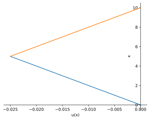
\(u_\text{AC} = -\cfrac{F \ x}{3 \ EA}\)
\(u_\text{BC} = -\cfrac{2 \ F \ L}{3 \ EA} + \cfrac{F \ x}{3 \ EA}\)
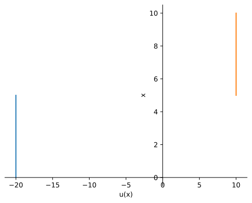
\(N_\text{AC} = -\cfrac{2 \ F}{3}\)
\(N_\text{BC} = -\cfrac{F }{3}\)

eq4 = sym.Eq(u_AC.subs(x,0), 0)
eq5 = sym.Eq(u_AC.subs(x,L), u_BC.subs(x,L))
eq6 = sym.Eq(u_BC.subs(x,2*L), 0)
eq7 = sym.Eq(N_AC.subs(x,L)+F, N_BC.subs(x,L))

display(eq4)
display(eq5)
display(eq6)
display(eq7)

C_sol = sym.solve((eq4,eq5,eq6,eq7),(C_1,C_2,C_3,C_4))
display(C_sol)

u_AC_sol = u_AC.subs(C_sol)
u_BC_sol = u_BC.subs(C_sol)
display(u_AC_sol)
display(u_BC_sol)
N_AC_sol = N_AC.subs(C_sol)
N_BC_sol = N_BC.subs(C_sol)
display(N_AC_sol)
display(N_BC_sol)

\[\displaystyle C_{2} = 0\]

\[\displaystyle \frac{C_{1} L}{2 EA} + C_{2} = \frac{C_{3} L}{EA} + C_{4}\]

\[\displaystyle \frac{2 C_{3} L}{EA} + C_{4} = 0\]

\[\displaystyle C_{1} + F = C_{3}\]

{C_1: -2*F/3, C_2: 0, C_3: F/3, C_4: -2*F*L/(3*EA)}

\[\displaystyle - \frac{F x}{3 EA}\]

\[\displaystyle - \frac{2 F L}{3 EA} + \frac{F x}{3 EA}\]

\[\displaystyle - \frac{2 F}{3}\]

\[\displaystyle \frac{F}{3}\]

%matplotlib inline
u_AC_func = sym.lambdify(x, u_AC_sol.subs(sol).subs(L,L_test).subs(EA,EA_test).subs(F,F_test))
u_BC_func = sym.lambdify(x, u_BC_sol.subs(sol).subs(L,L_test).subs(EA,EA_test).subs(F,F_test))
x_plot_AC = np.linspace(0, L_test,100)
x_plot_BC = np.linspace(L_test, L_test*2,100)
fig, ax = plt.subplots()
ax.plot(u_AC_func(x_plot_AC),x_plot_AC)
ax.plot(u_BC_func(x_plot_BC),x_plot_BC)
ax.spines['right'].set_color('none')
ax.spines['top'].set_color('none')
ax.spines['bottom'].set_position('zero')
ax.spines['left'].set_position('zero')
ax.set_xlabel('u(x)')
ax.set_ylabel('x')
fig.patch.set_alpha(0.0)
ax.patch.set_alpha(0.0)

../_images/e1b7d72388ee9cae0d7443b63b0bd907978beb9b026fbd8a82d4a6a691b71451.svg

N_AC_func = sym.lambdify(x, N_AC_sol.subs(L,L_test).subs(EA,EA_test).subs(F,F_test))
N_BC_func = sym.lambdify(x, N_BC_sol.subs(L,L_test).subs(EA,EA_test).subs(F,F_test))
x_plot_AC = np.linspace(0, L_test,2)
x_plot_BC = np.linspace(L_test, L_test*2,2)
fig, ax = plt.subplots()
ax.plot(N_AC_func(x_plot_AC)*np.ones(2),x_plot_AC)
ax.plot(N_BC_func(x_plot_BC)*np.ones(2),x_plot_BC)
ax.spines['right'].set_color('none')
ax.spines['top'].set_color('none')
ax.spines['bottom'].set_position('zero')
ax.spines['left'].set_position('zero')
ax.set_xlabel('u(x)')
ax.set_ylabel('x')
fig.patch.set_alpha(0.0)
ax.patch.set_alpha(0.0)

../_images/681bc7a56b2d05edff0544c8192e02840e7e992b35226eacd9b8c9e85930a1b2.svg

Comparison#

Now, let’s compare the plots of both solution strategies, you can try different values:

from ipywidgets import widgets, interact

%matplotlib widget

fig, ax = plt.subplots()
fig.canvas.toolbar_visible = False
def func(L_test, EA_test, F_test):
    ax.clear()
    u_trial_func = sym.lambdify(x, u_trial_sol.subs(sol).subs(L,L_test).subs(EA,EA_test).subs(F,F_test))
    u_AC_func = sym.lambdify(x, u_AC_sol.subs(sol).subs(L,L_test).subs(EA,EA_test).subs(F,F_test))
    u_BC_func = sym.lambdify(x, u_BC_sol.subs(sol).subs(L,L_test).subs(EA,EA_test).subs(F,F_test))
    x_plot = np.linspace(0, L_test*2,100)
    x_plot_AC = np.linspace(0, L_test,2)
    x_plot_BC = np.linspace(L_test, L_test*2,2)
    ax.plot(u_AC_func(x_plot_AC),x_plot_AC,label='u_AC ODE')
    ax.plot(u_BC_func(x_plot_BC),x_plot_BC, label='u_BC ODE')
    ax.plot(u_trial_func(x_plot),x_plot, label='u trial')
    ax.spines['right'].set_color('none')
    ax.spines['top'].set_color('none')
    ax.spines['bottom'].set_position('zero')
    ax.spines['left'].set_position('zero')
    ax.set_xlabel('u(x)')
    ax.set_ylabel('x')
    ax.legend(loc='best')
    fig.patch.set_alpha(0.0)
    ax.patch.set_alpha(0.0)

interact(func, L_test = widgets.FloatSlider(min=0.1, max=5, value=2, step=0.1, description="Length (m)",readout_format='.1f',style= {'description_width': '200px'},layout = {'width': '450px'}),
         EA_test = widgets.FloatSlider(min=1000, max=10000, value=2000, step=100, description="EA (kN)",readout_format='.1f',style= {'description_width': '200px'},layout = {'width': '450px'}),
         F_test = widgets.FloatSlider(min=10, max=100, value=30, step=1, description="Force (kN)",readout_format='.1f',style= {'description_width': '200px'},layout = {'width': '450px'}) );

%matplotlib widget
fig, ax = plt.subplots()
fig.canvas.toolbar_visible = False

def func(L_test, EA_test, F_test):
    ax.clear()
    N_trial_func_AC = sym.lambdify(x, N_trial_sol_AC.subs(L,L_test).subs(EA,EA_test).subs(F,F_test))
    N_trial_func_BC = sym.lambdify(x, N_trial_sol_BC.subs(L,L_test).subs(EA,EA_test).subs(F,F_test))
    N_AC_func = sym.lambdify(x, N_AC_sol.subs(L,L_test).subs(EA,EA_test).subs(F,F_test))
    N_BC_func = sym.lambdify(x, N_BC_sol.subs(L,L_test).subs(EA,EA_test).subs(F,F_test))
    x_plot = np.linspace(0, L_test*2,2)
    x_plot_AC = np.linspace(0, L_test,2)
    x_plot_BC = np.linspace(L_test, L_test*2,2)
    ax.plot(N_AC_func(x_plot_AC)*np.ones(2),x_plot_AC,label='u_AC ODE')
    ax.plot(N_BC_func(x_plot_BC)*np.ones(2),x_plot_BC, label='u_BC ODE')
    ax.plot(N_trial_func_AC(x_plot_AC),x_plot_AC, label='u_AC trial')
    ax.plot(N_trial_func_BC(x_plot_BC),x_plot_BC, label='u_BC trial')
    ax.spines['right'].set_color('none')
    ax.spines['top'].set_color('none')
    ax.spines['bottom'].set_position('zero')
    ax.spines['left'].set_position('zero')
    ax.set_xlabel('N(x)')
    ax.set_ylabel('x')
    ax.legend(loc='best')
    fig.patch.set_alpha(0.0)
    ax.patch.set_alpha(0.0)

interact(func, L_test = widgets.FloatSlider(min=0.1, max=5, value=2, step=0.1, description="Length (m)",readout_format='.1f',style= {'description_width': '200px'},layout = {'width': '450px'}),
         EA_test = widgets.FloatSlider(min=1000, max=10000, value=2000, step=100, description="EA (kN)",readout_format='.1f',style= {'description_width': '200px'},layout = {'width': '450px'}),
         F_test = widgets.FloatSlider(min=10, max=100, value=30, step=1, description="Force (kN)",readout_format='.1f',style= {'description_width': '200px'},layout = {'width': '450px'}) );

Exercise (Comparison)

Would you consider the trial function solution for proper estimates for displacements? How about normal forces?

Solution to Exercise (Comparison)

The estimation for displacement seems okayish, but the difference with the ‘real’ solution for normal force distribution is much bigger so it might not be advised to use that.

Exercise potential energy statically indeterminate structure

Contents

Exercise potential energy statically indeterminate structure#

Solve using potential energy#

Solve with differential equation#

Comparison#