Matrixframe

Matrixframe is commercial software for structural analysis. MatrixFrame uses symbols that closely resemble those used in the curriculum at Delft. For students, there is a free student license (registration with MatrixFrame required) and a version that only works on the TU Delft network (possibly via VPN connection). If you have requested the student license but have not received it, you can submit a ticket via this link.

A few important points when using MatrixFrame:

• When using MatrixFrame, you must always enter the stiffness of the elements (‘profile data in MatrixFrame’). MatrixFrame needs this information to perform the calculations, even if it is not necessary for the force quantities in statically determinate structures. If these data are unknown, you can enter a large arbitrary value under ‘Manual input’ to model an infinitely stiff bar. If the value is several orders of magnitude larger than the other values, it is sufficient; if the value is too large, numerical issues may arise.

• Sometimes elements can overlap without you noticing.

A comprehensive manual with more options can be found here. The official documentation also provides more explanation.

In general, the following steps are required:

Algorithm (Input and output of a structure in MatrixFrame)

1. Create a new project - ‘2D-Raamwerk’ and click ‘Ok’. The options ‘1D-ligger’ and ‘2D-vakwerk’ are simplifications of the ‘2D-Raamwerk’ option. You can try the ‘3D-Raamwerk’ and ‘3D-Vakwerk’ options, but these are generally more complex.

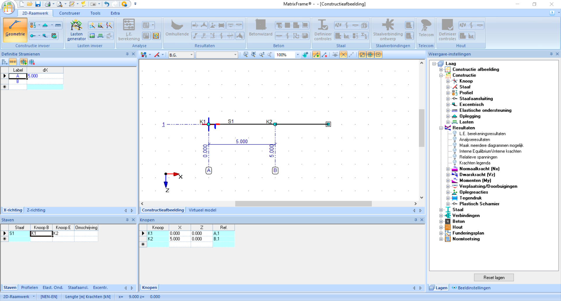
2. You enter the ‘Geometrie’ interface. Click in the grid to create your geometry. The coordinates are visible in the bottom bar and the dimensions appear while clicking. Use Esc on your keyboard to stop or to start a new element that is not attached to the end of the previous element. Optionally, adjust dimensions using the grids on the left or the coordinates at the bottom of the screen.

3. Continue with the ‘Profielgegevens’ interface. Even if this information is unknown, entering it is required. Under ‘Profielen’ - ‘Handmatige invoer’ you can enter \(A\), \(I\), and \(E\). It is not possible to enter a value of \(0\) or \(\infty\); instead, enter a small or large numerical value. Tip: \(\cdot10^6\) can be entered as e6. Don’t forget to click ‘Pas toe op alles’! In the lower left of the screen, you will now see a profile name behind each bar.

4. The next step is adding supports. There are several standard options, but you can also manually fix translation and rotation directions. Supports can be placed on the nodes or alongside elements (in that case a new node is created).

5. Next, we can add hinges. In a raamwerk, everything is moment-fixed by default. For each member, you can indicate for each end whether it should be a scharnier by clicking on part of that member. If two connecting staven are scharnierend, it is not necessary to hinge both member ends; one is enough.

6. The last configuration step is adding loads. You can add different belastingsgevallen (B.G.), but if you only need to calculate one, it is not necessary to adjust these options. For each belasting, you must specify the value and direction and click the member on which the load acts. In the venster at the bottom of the screen, you can also adjust these.

7. Now that everything is configured, you can click on ‘L.E. berekening’ (linear-elastic calculation). A dialog window will open that gives error messages if something is incorrect.

8. To view the results, there are several options. The reaction forces can be shown separately. Note: the direction of the arrows indicates the actual direction of the forces and moments; a minus sign indicates that the force acts in the negative direction of the coordinate system.

9. The internal force diagrams can also be shown. These can be displayed per internal force according to the deformation symbols as we are used to. If the deformation symbols are not visible, you can zoom in or increase the scale under ‘Weergave-instellingen’ - ‘Beeldinstellingen’ - ‘Eigenschappen’ - ‘Resultaten’ - ‘Normaalkracht (Nx)’/’Dwarskracht (Vz)’/’Moment (My)’ - ‘Vorm’ - ‘Schaal’ - Enter value and click ‘Toepassen’. If a member is clicked, all internal forces and displacements of that member are visible on the left of the screen. At the bottom of the screen, several characteristic values are shown. The values are shown according to the local coordinate system.

10. Displacements can also be shown. The number of decimals can be adjusted under ‘Weergave-instellingen’ - ‘Beeldinstellingen’ - ‘Eigenschappen’ - ‘Resultaten’ - ‘Verplaatsingen/Doorbuigingen’ - ‘Label’ - ‘Decimalen’ - Enter value and click ‘Toepassen’.

11. Finally, values at specific positions can be read using the spion functie. Click a member and enter a location under ‘Invoer pos:’ in the local coordinate system. The table and graphical display then show values of internal forces and displacements at that point.

As an example, we determine the external static indeterminacy of this structure.

Example

Fig. 80 Example structure

1. Create a new project - ‘2D-Raamwerk’ and click ‘Ok’. The options ‘1D-ligger’ and ‘2D-vakwerk’ are simplifications of the ‘2D-Raamwerk’ option. You can try the ‘3D-Raamwerk’ and ‘3D-Vakwerk’ options, but these are generally more complex.

   Example

   

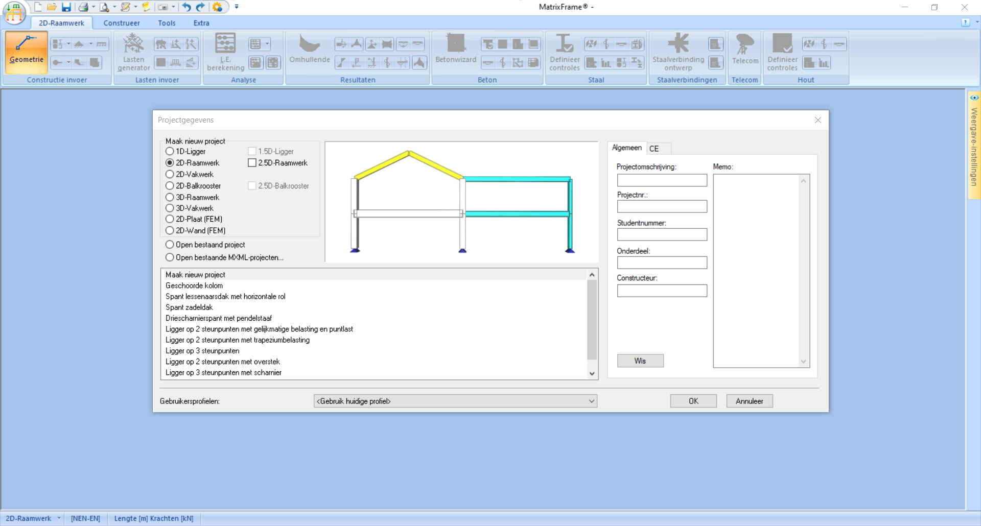
   Fig. 81 Since this is a 2D frame, we select that option.

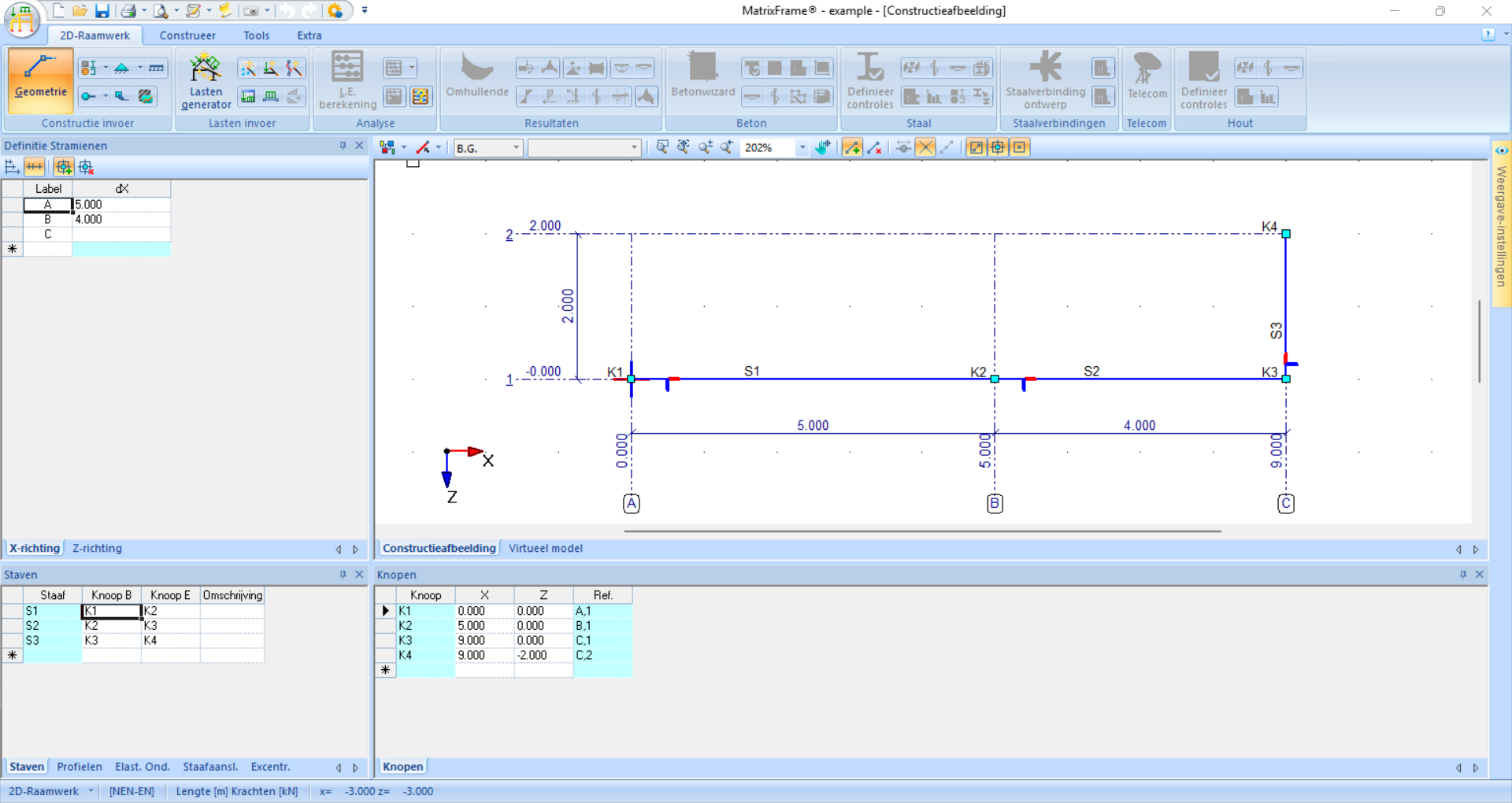
2. You enter the ‘Geometrie’ interface. Click in the grid to create your geometry. The coordinates are visible in the bottom bar and the dimensions appear while clicking. Use Esc on your keyboard to stop or to start a new element that is not attached to the end of the previous element. Optionally, adjust dimensions using the grids on the left or the coordinates at the bottom of the screen.

   Example

   

   Fig. 82 The first bar has already been drawn and for the second bar, the coordinate \(\left(9,0 \right)\) is visible in the bar at the bottom.

   

   Fig. 83 This is the result when all nodes and bars have been drawn.

3. Continue with the ‘Profielgegevens’ interface. Even if this information is unknown, entering it is required. Under ‘Profielen’ - ‘Handmatige invoer’ you can enter \(A\), \(I\), and \(E\). It is not possible to enter a value of \(0\) or \(\infty\); instead, enter a small or large numerical value. Tip: \(\cdot10^6\) can be entered as e6. Don’t forget to click ‘Pas toe op alles’! In the lower left of the screen, you will now see a profile name behind each bar.

   Example

   In this example, only an \(EI\) value is given, while we need to enter separate \(E\) and \(I\) values. Therefore, you can choose two numbers whose product is \(7.8 \cdot 10^4\), for example, \(E = 200 \cdot 10^6\) and \(I = 3.9 \cdot 10^-2\). \(EA\) is \(\infty\), for which we can enter a large numerical value, for example, \(A = 10 \cdot 10^3\).

   

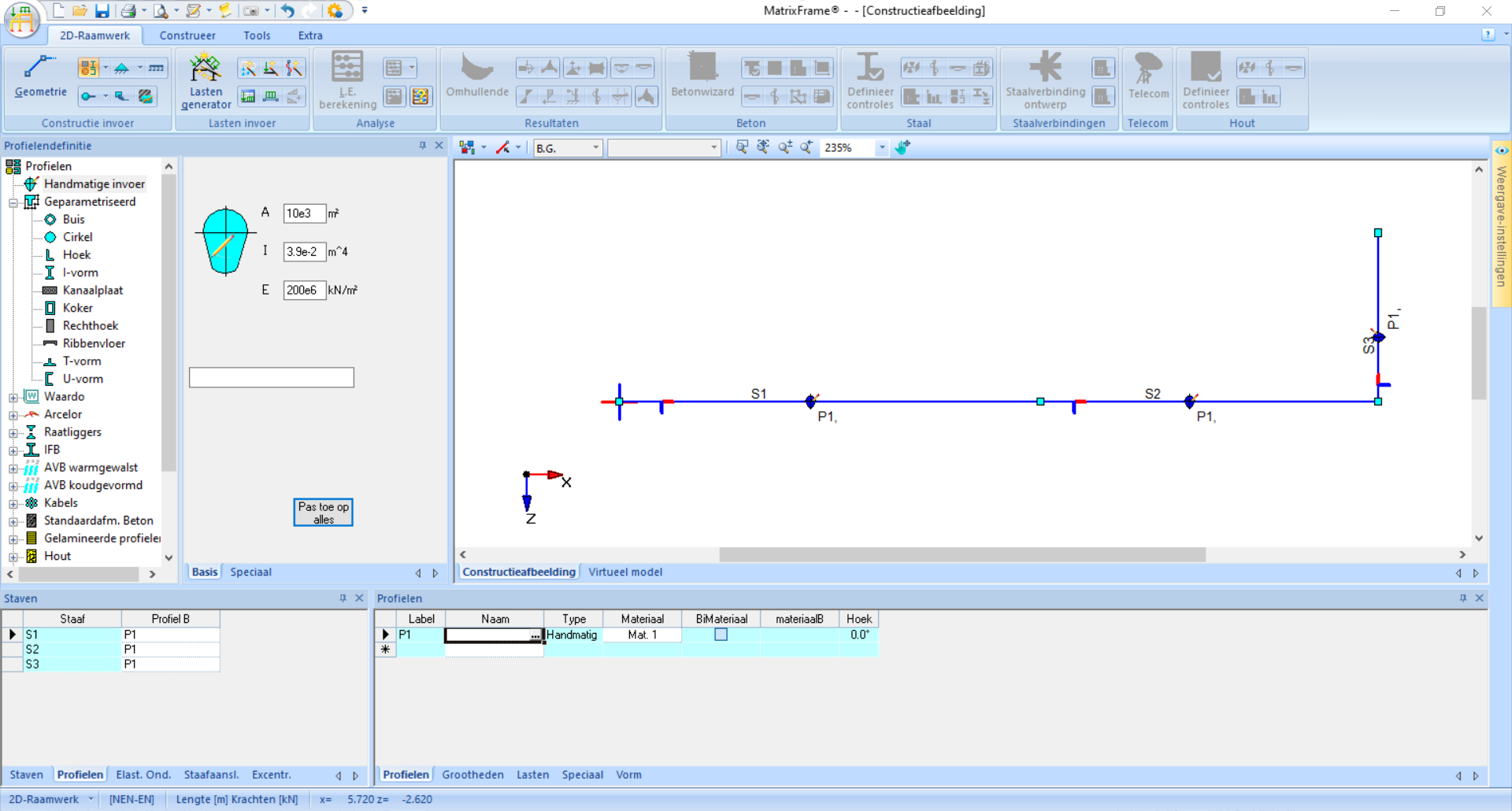
   Fig. 84 If everything is entered, this is the result.

4. The next step is adding supports. There are several standard options, but you can also manually fix translation and rotation directions. Supports can be placed on the nodes or along a bar (in that case a new node is created).

   Example

   

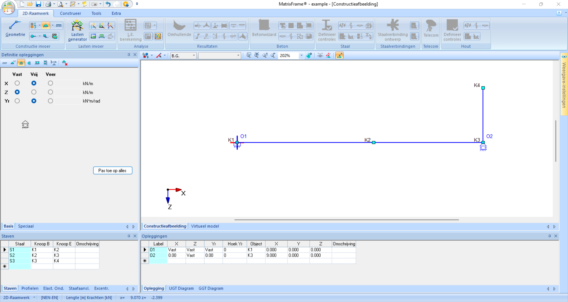
   Fig. 85 The fixed support and roller support of the example are visible in both the graphical display and the lower window after being added.

5. Next, we can add hinges. In a raamwerk, everything is moment-fixed by default. For each staaf, you can indicate for each end whether it should be a scharnier by clicking on part of that staaf. If two connecting staven are scharnierend, it is not necessary to hinge both staaf ends; one is enough.

   Example

   

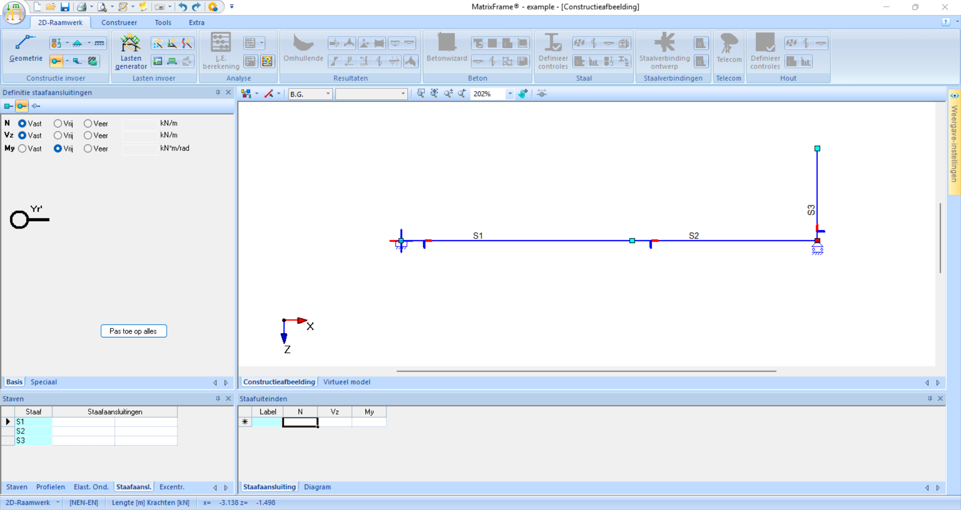
   Fig. 86 In this example, there are no hinges, so this step can be skipped.

6. The last configuration step is adding loads. You can add different loading cases (B.G.), but if you only need to calculate one, it is not necessary to adjust these options. For each load, you must specify the value and direction and click the bar on which the load acts. In the window at the bottom of the screen, you can also adjust these.

   Example

   

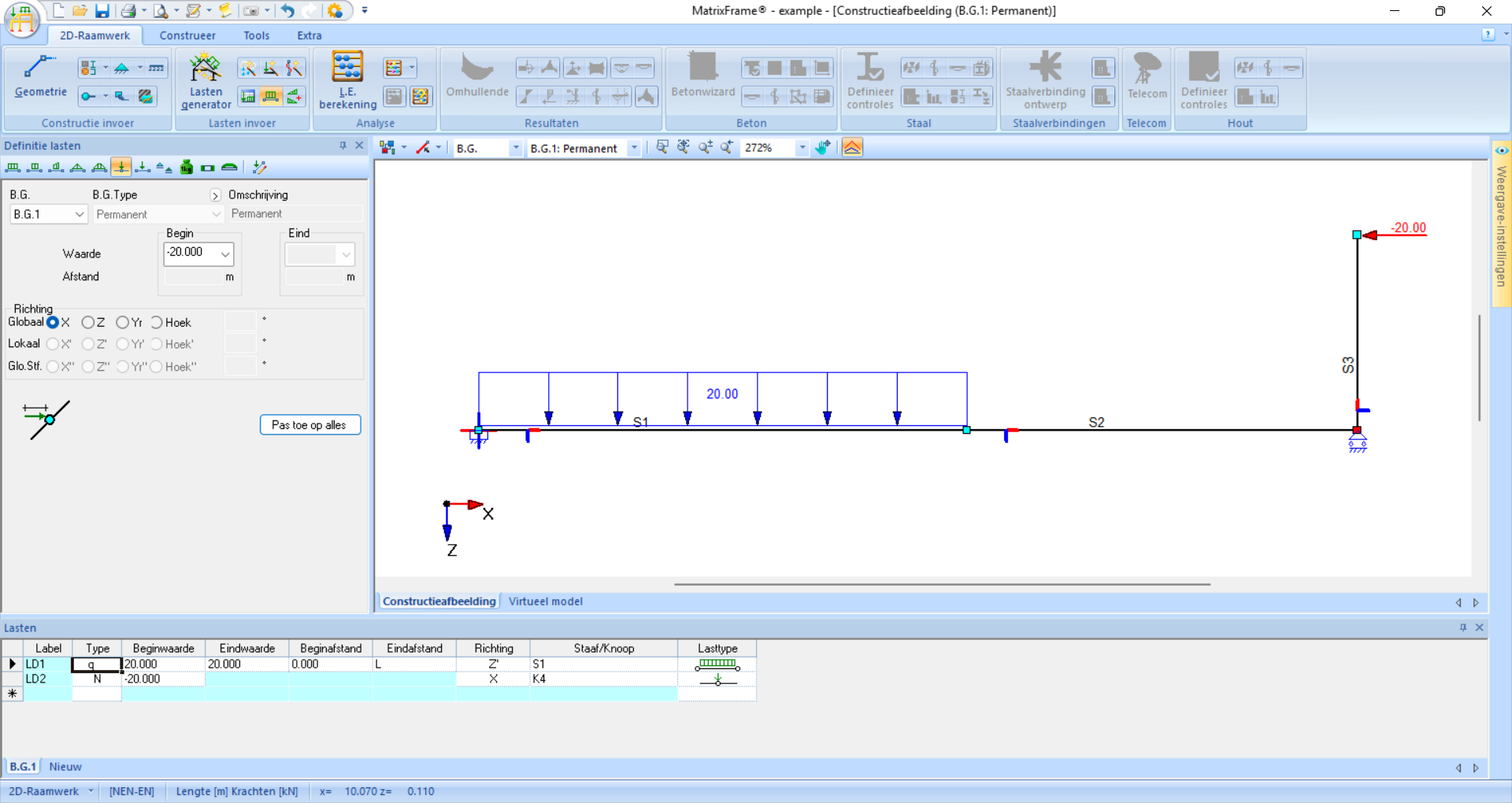
   Fig. 87 In this example, there are two loads. The distributed load is applied in the local z-direction and the point load in the global x-direction with a negative value so that it acts to the left.

7. Now that everything is configured, you can click on ‘L.E. berekening’ (linear-elastic calculation). A dialog window will open that gives error messages if something is incorrect.

   Example

   

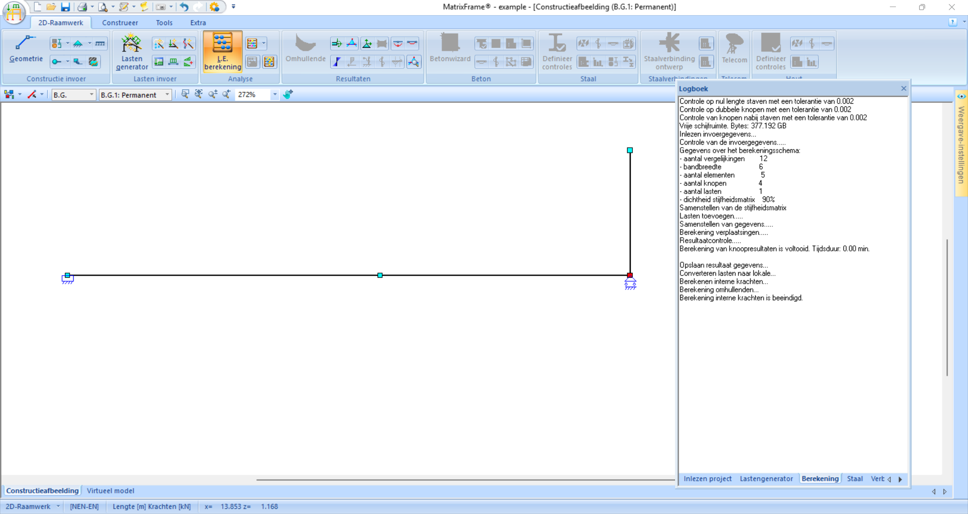
   Fig. 88 In this example, everything is configured correctly and the logbook shows no error messages.

8. To view the results, there are several options. The support reactions can be shown separately. Note: the direction of the arrows indicates the actual direction of the forces and moments; a minus sign indicates that the force acts in the negative direction of the coordinate system.

   Example

   

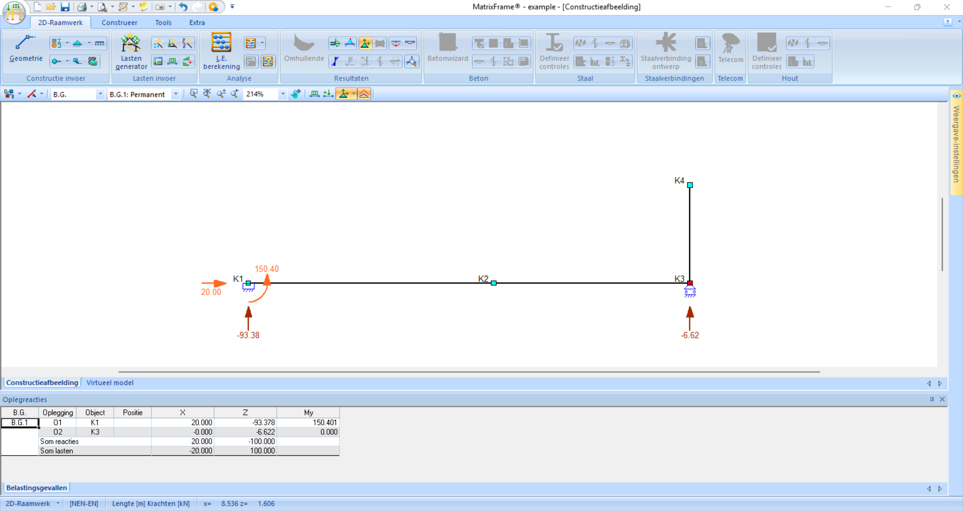
   Fig. 89 In this example, four support reactions are visible. The vertical support reactions act upwards; the minus sign indicates that these act in the negative z-direction.

9. The internal force distributions can also be shown. These can be displayed per internal force according to the deformation symbols as we are used to. If the deformation symbols are not visible, you can zoom in or increase the scale under ‘Weergave-instellingen’ - ‘Beeldinstellingen’ - ‘Eigenschappen’ - ‘Resultaten’ - ‘Normaalkracht (Nx)’/’Dwarskracht (Vz)’/’Moment (My)’ - ‘Vorm’ - ‘Schaal’ - Enter value and click ‘Toepassen’. If a bar is clicked, all internal forces and displacements of that bar are visible on the left of the screen. At the bottom of the screen, several characteristic values are shown. The values are shown according to the local coordinate system.

   Example

   

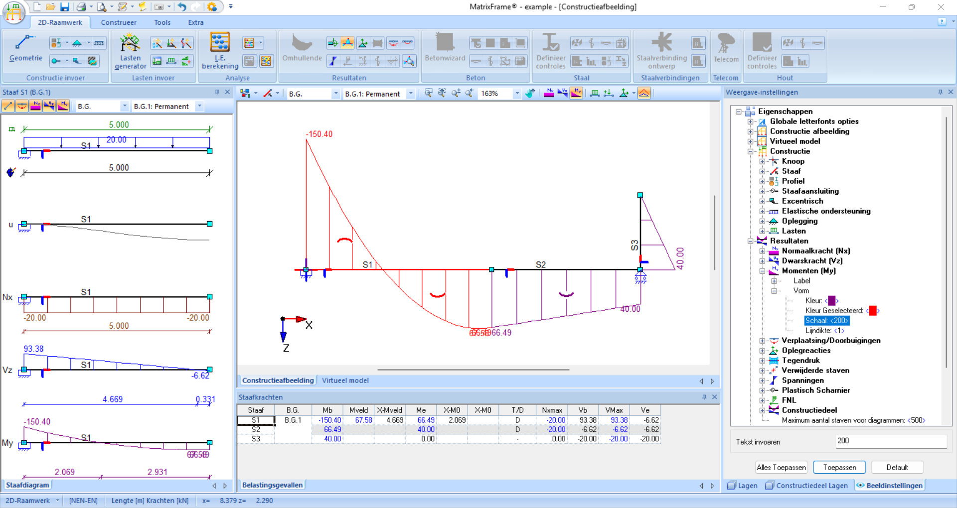
   Fig. 90 The moments have been made visible with bar AD in detail on the left. The scale has been adjusted so that the deformation symbols are visible.

   

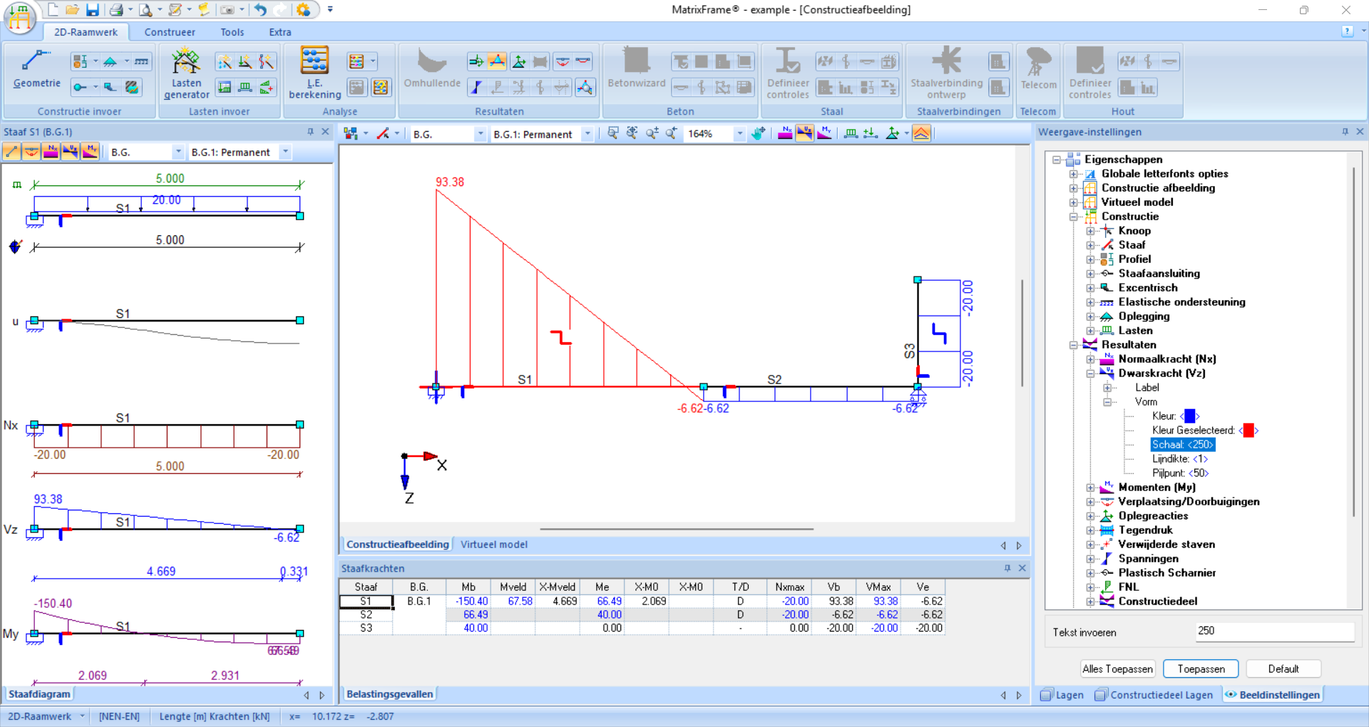
   Fig. 91 Also, the shear forces can be displayed. The deformation symbol of DB is not visible in this view; if you zoom in further or increase the scale further, it would become visible. The normal forces can also be made visible.

   

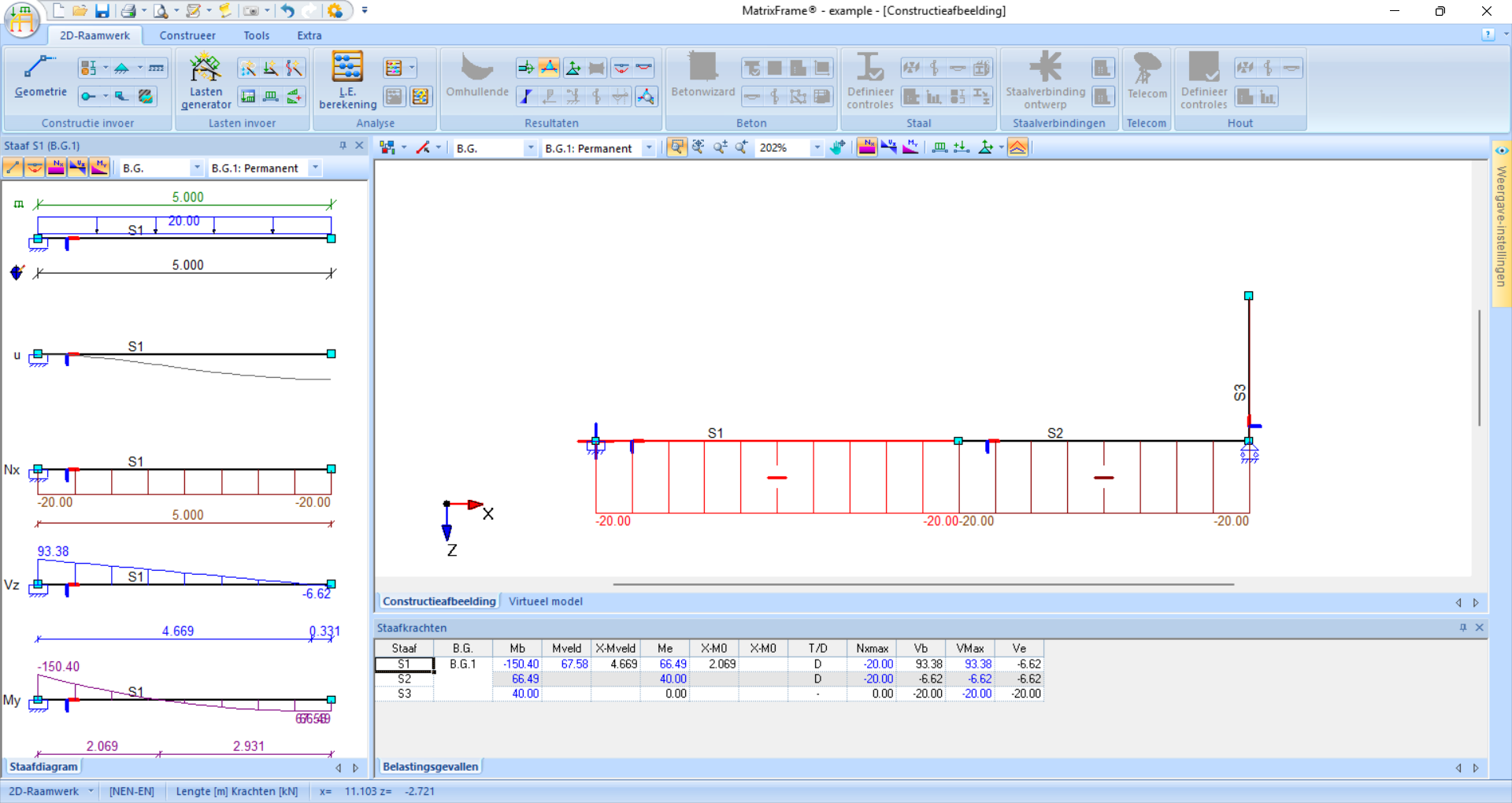
   Fig. 92 The normal forces can also be made visible.

10. Displacements can also be shown. The number of decimals can be adjusted under ‘Weergave-instellingen’ - ‘Beeldinstellingen’ - ‘Eigenschappen’ - ‘Resultaten’ - ‘Verplaatsingen/Doorbuigingen’ - ‘Label’ - ‘Decimalen’ - Enter value and click ‘Toepassen’

    Example

    

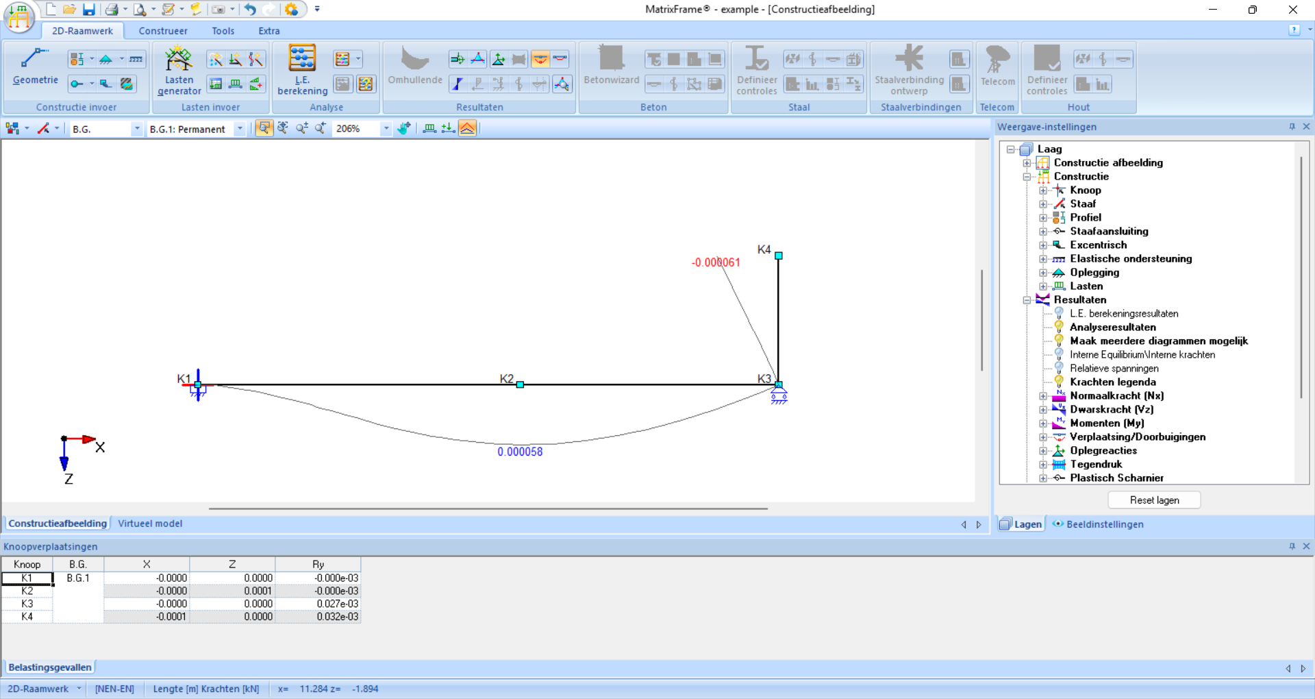
    Fig. 93 The displacements have been made visible. The number of decimals has been adjusted so that the exact displacements can be found.

11. Finally, values at specific positions can be read using the spion functie. Click a member and enter a location under ‘Invoer pos:’ in the local coordinate system. The table and graphical display then show values of snedekrachten and verplaatsingen at that point.

    Example

    

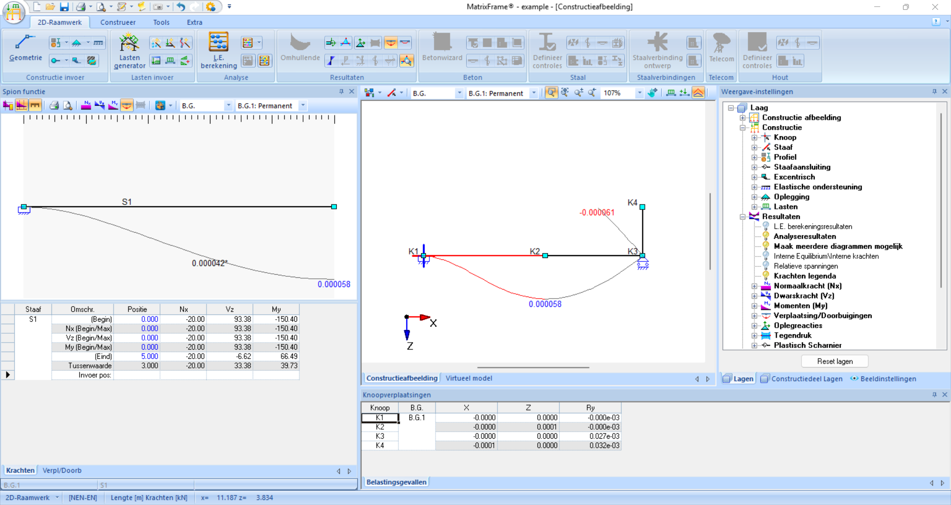
    Fig. 94 At \(3\) meters to the right of A, the snedekrachten and verplaatsingen have been determined for this example: a displacement of \(0.000042 \ \rm{m}\), a moment of \(39.73 \ \rm{kNm}\), a shear force of \(33.38 \ \rm{kN}\), and a normal force of \(-20 \ \rm{kN}\).

Example

The file of this example can be downloaded here.

Instructions from lecture

This example is presented in a lecture available here for TU Delft students.